The Carbon Budget Analysis Tool (CBAT)
Click logo to return to 'CBAT-general-page'
CBAT Domain 1 - Contraction & Concentrations (keeping or losing control)?
CBAT Appreciation
This is the CBAT Domain 1, the module for the cognitive mapping of positive feedback potential and control . . .
Consider the image below for user-controls & then click the image below to get to the real-time user-chooser animation
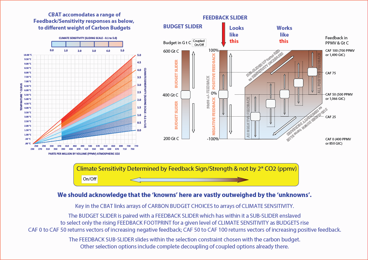
Rationalizing 'feedback-dynamics' (the monster in the model) means mathematizing unknowns (both known & unknown).
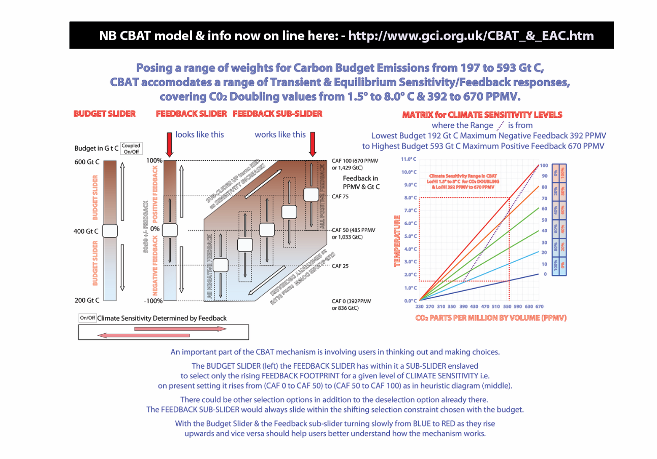
In CBAT, the known & the unknown-unknowns concerning the sign (+/-) & the extent of feedback rates, are rationalized in the following way.
The Constant Airborne Fraction of CO2 emissions (CAF) is a key 'reference-value' used in CBAT.
CAF-50 has been set at 50% in CBAT as CAF 50 is what we are presently at
This method simply: -
- reflects that as things now stand, every two years the atmosphere retains roughly the equivalent of 100% of one year's CO2 emissions.
- enables the 'feedback control' slider (slider D) to be chosen by the user set to reflect the extent to which any future CAF may be either: -
- below CAF-50 (overall negative feedback) or
- above CAF-50 (overall positive feedback)
*************************************************************************
CBAT Domain One is the basis of all four Domains in CBAT; all Domains are user-interactive.
Within the structure described below, CBAT Domain One embodies the crucial distinction between: -
- Budget emissions/atmosphere-concentrations (effectively feedback-free modelling) and
- Feedback emissions-effects/atmosphere-concentrations (which increasingly can amplify the climate-effects above budget-emissions/concentrations).
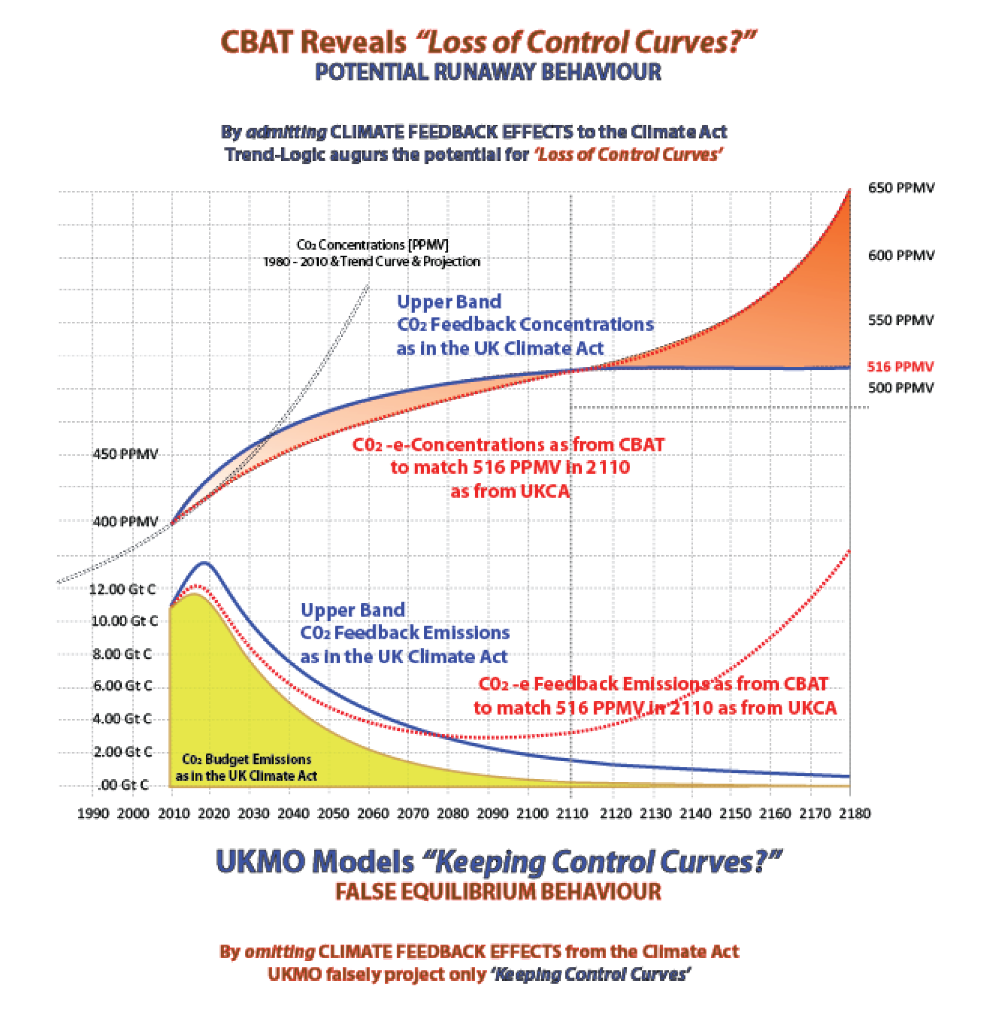
Considerable detail about this was provided to the EAC Enquiries into 'Carbon Budgets in the UK Climate Act' in 2009 & 2013.
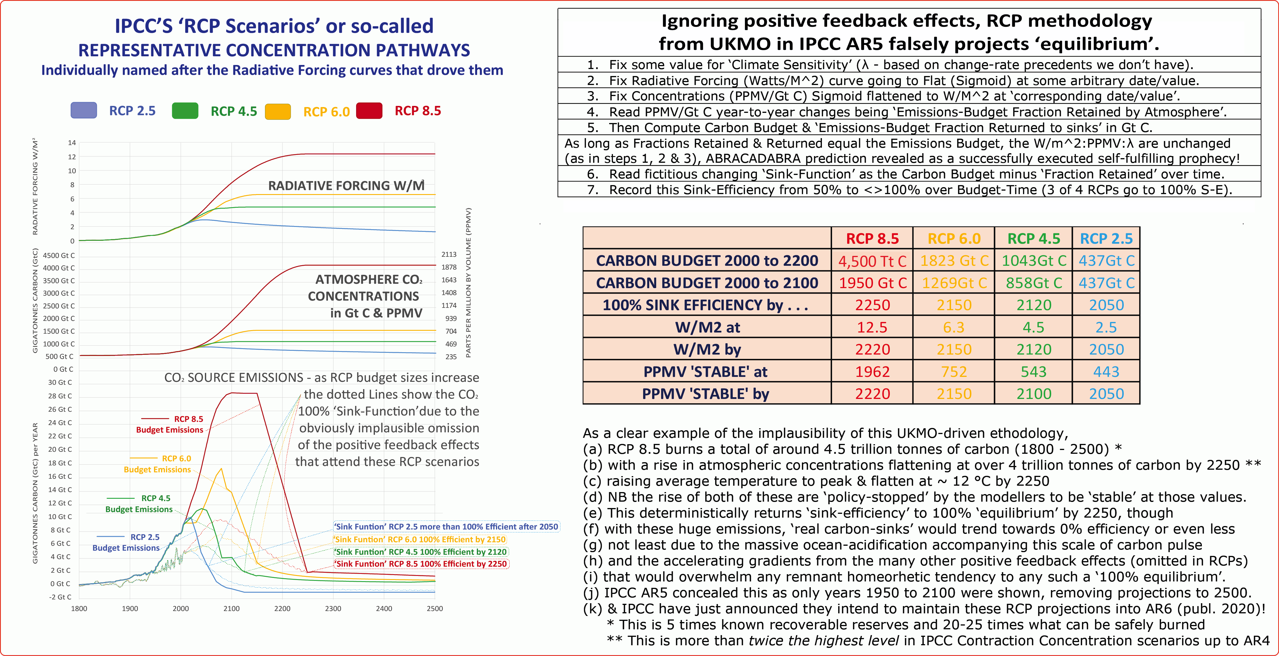
It was pretty obvious that generically, the UKMO treatment of this huge subject was constrained by false equilibrium
assumptions that were seriously misleading, due to the failure to engage with the imminent positive feedback-crisis.
*************************************************************************
CBAT Domain One
Contraction & Concentrations Budget-Emissions without feedback gives 'keeping control' curvature
Using carbon-cycle climate models, budget emissions/concentrations are what climate modellers have tended mainly to focus on in the past. These are relatively easy to model/project,
as budget emissions are measured as 'human' emissions from Oil, Coal, Gas and Land-Use Change & the 'known-unknowns' of feedback emissions-effects had been largely omitted.
The modelling assumption has been that as atmospheric concentrations have always been a 'Constant Airborne Fraction' of emissions at around 50% of emissions (CAF 50) in the past,
this will continue in future. In CBAT as & if budget emissions fall, the rise of concentrations will slow as CAF 50 decreases, & start to fall if budget emissions go to zero rapidly.In this modelling paradigm of 'climate control', 'climate-scientist's' cut out all the unknowns about feedbacks & the inter-activity of the rates of feedback & hence uncertainty about these.
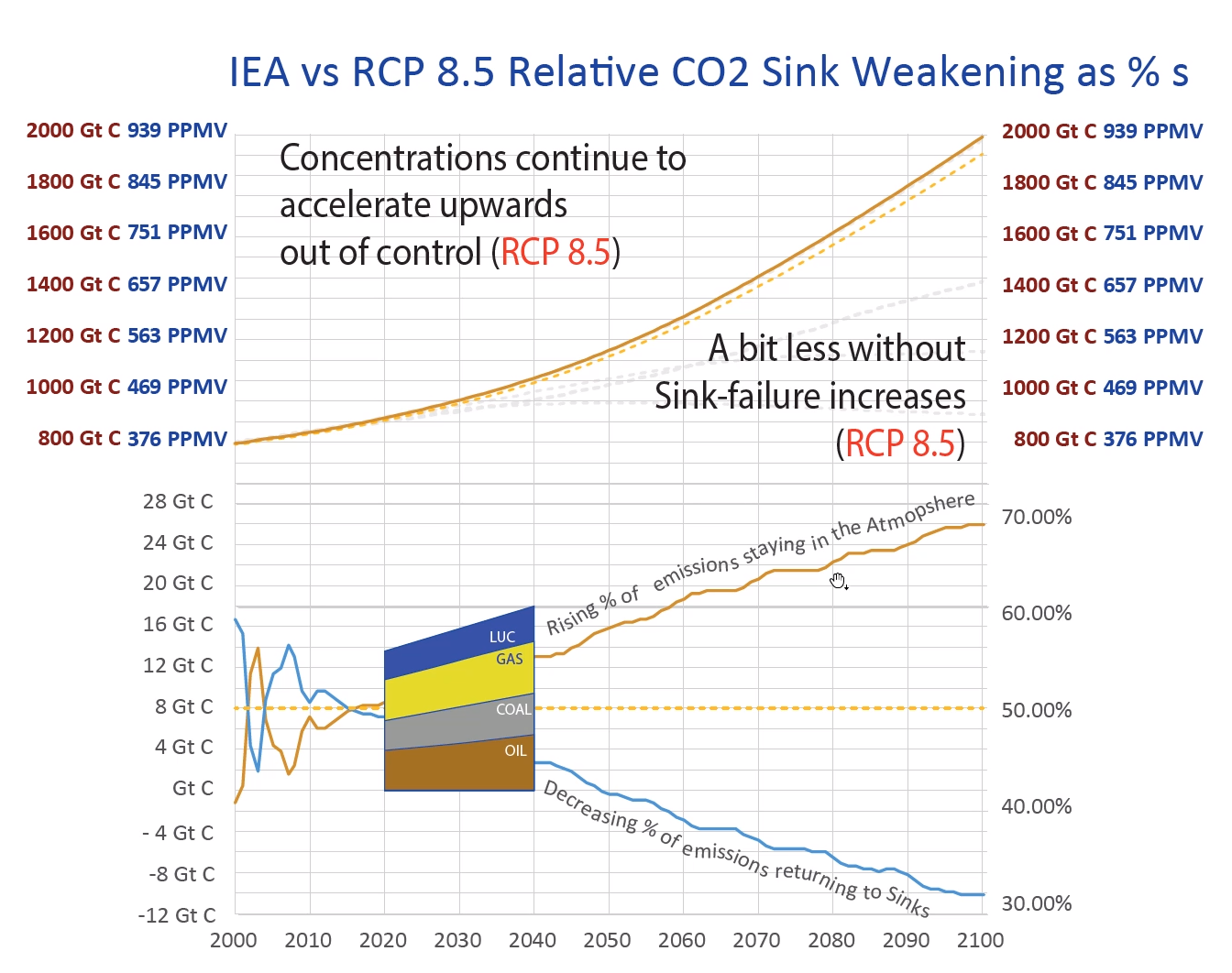
So below CAF 50, the curve-shape of concentrations is convex, where deceleration shows keeping-control-curvature. Ridiculously, this was mapped on all of the RCP Scenarios in IPCC AR5.
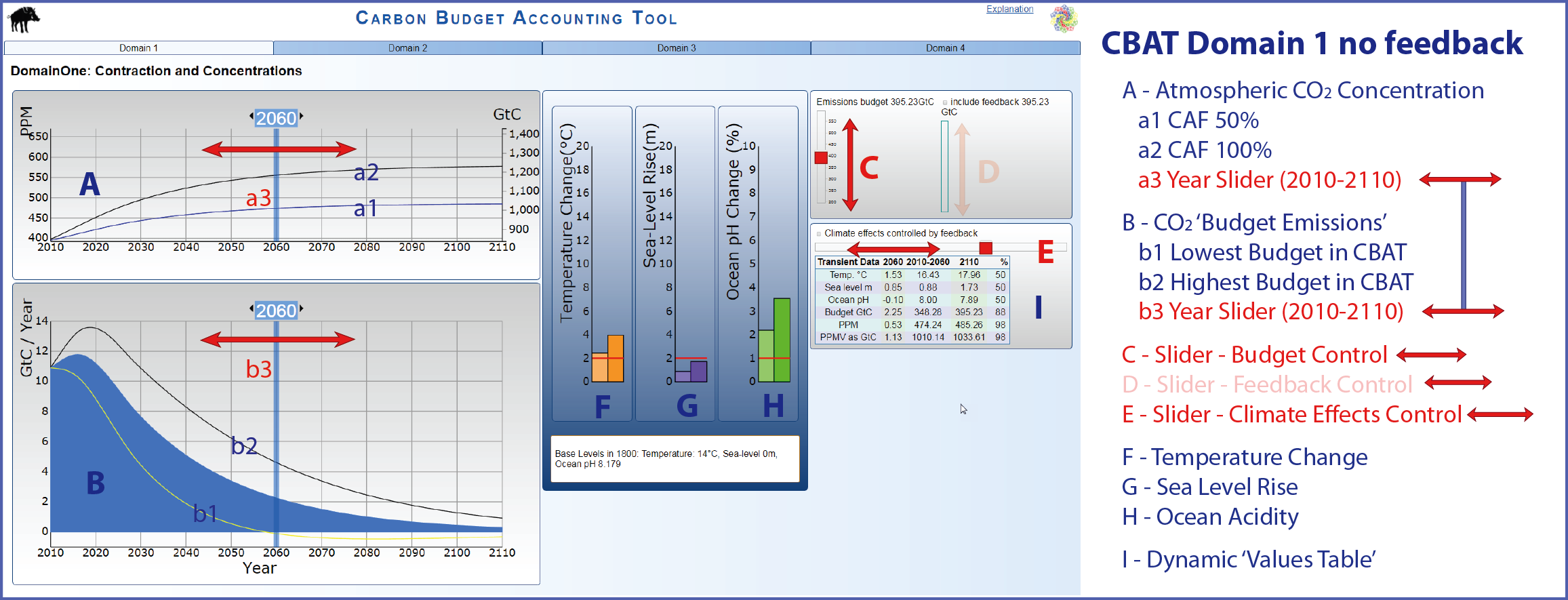
- A - Atmospheric CO2 Concentration
- a1 CAF 50% (to cross-reference emissions:concentrations - 1 PPMV CO2 equals 2.13 Gt C)
- a2 CAF 100% (to cross-reference emissions:concentrations - 1 PPMV CO2 equals 2.13 Gt C)
- a3 Year Slider 2010-2110 (NB a3 & b3 are deliberately locked together)
- B - CO2 ‘Budget Emissions’
- b1 Lowest Budget in CBAT
- b2 Highest Budget in CBAT
- b3 Year Slider 2010-2110 (NB a3 & b3 are deliberately locked together)
- C - Slider - Budget Control
- D - Slider - Feedback Control
- E - Slider - Climate Effects Control for a range of potential effects wider than considered in the IPCC.
These measure wider with the amplification of climate effects on the enslaved: -
- F - Temperature Change (left-hand bar time-transient to right-hand bar outcome value in 2110)
- G - Sea Level Rise (left-hand bar time-transient to right-hand bar outcome value in 2110)
- H - Ocean Acidity ((left-hand bar time-transient to right-hand bar outcome value in 2110)
- I - Dynamic ‘Values Table’
The left-hand slider in the panel top right-hand corner varies the 'carbon-weight'. Covering the period 2010 to 2110 Gt C, the integral-weight
of the 'global carbon budget' in Domain 1 (as with all 4 CBAT Domains) ranges between 197 to 593 Gt C.
The blue chart on the left at the bottom drawing CO2 emissions, responds to the budget slider between the lower and upper limits shown.
The lines chart above shows atmospheric CO2 concentrations with budget-emissions accumulating at a constant 50% and at a constant 100%.
The table below the sliders is dynamic. All the numbers shown will always correspond with the carbon-weight of the budget-emissions chosen with the slider etc.
If a budget of 400 Gt C is chosen (see above the slider), the bottom right-hand column of the table will also show 400Gt C at 2100 and so on.
CBAT Domain 1
Contraction & Concentrations Feedback Emissions gives potential 'loss of control' curvatureWhen potential feedback emissions/concentrations/effects are added, the key curve-shape gradually gives way to convex or acceleration curvature.
In this modelling paradigm of 'loss of climate control', the unknowns about feedbacks & the inter-activity of the rates of feedback & hence uncertainty about these are included. i.e above CAF 50,
the curve-shape of concentrations is increasingly convex, where acceleration shows loss-of-control-curvature. This obvious concern was not mapped into any of the RCP Scenarios in IPCC AR5.
Once feedback effects take hold, more warming becomes locked in & there is little we can do about this. So in this modelling paradigm, uncertainties, unknowns & unknowability' mean that unless 'budget-emissions control' is very tight from now on, we inevitably face an increasing 'loss of climate control' and the increase of risks & actual damages.
This goes beyond the "careful & ultra-conservative feedback-modelling" (1:02:08) published in the IPCC over the last 30 years.
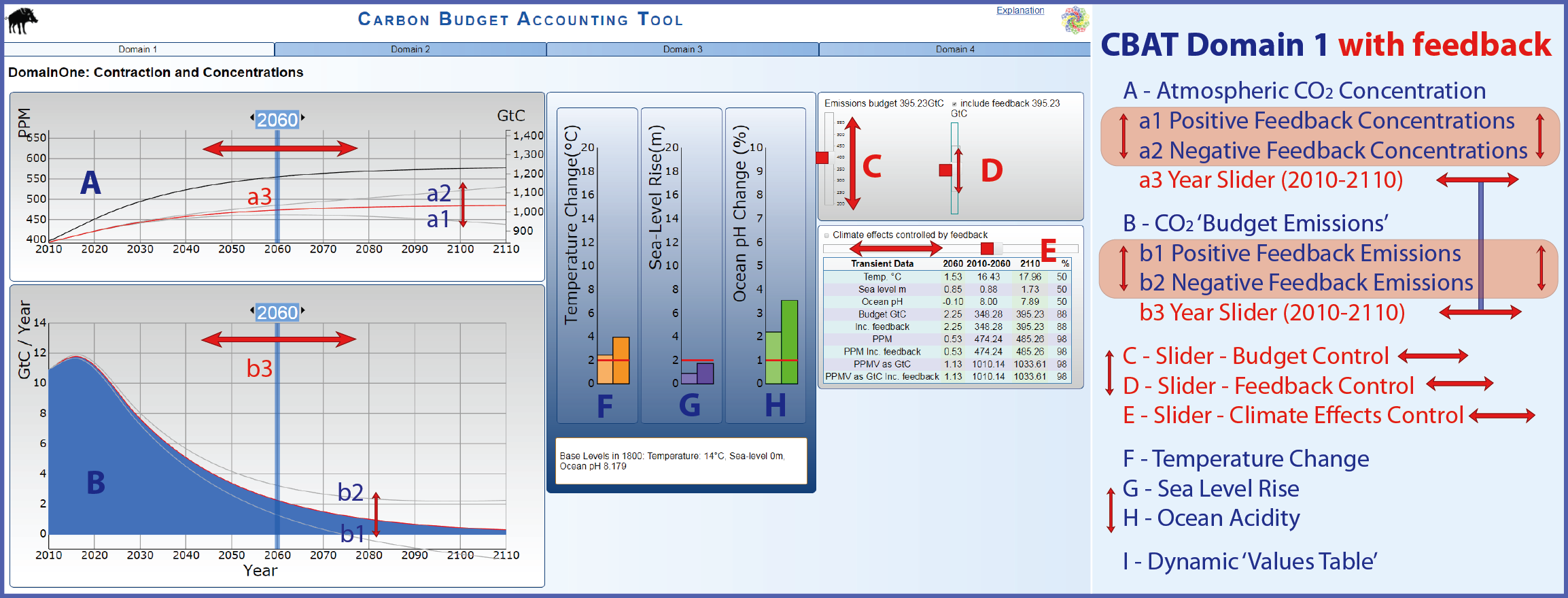
The right-hand slider in the panel top right-hand corner varies the 'carbon-weight'. Covering the period 2010 to 2110 Gt C, the integral-weight
- A - Atmospheric CO2 Concentration potential ranges between
- a1 Positive-Feedback Concentrations
- a2 Negative-Feedback Concentrations
- a3 Year Slider 2010-2110 (NB a3 & b3 are deliberately locked together)
- B - CO2 ‘Feedback Emissions’ potential ranges between
- b1 Positive-Feedback Emissions
- b2 Negative-Feedback Emissions
Note that the bigger the Budget Emissions total, the more likely the net feedback
effect triggered is 'positive' i.e. showing 'acceleration - or loss of control - curvature'.
In other words as the Emission Budget total increases, the 'positive feedback potential' does too.
- b3 Year Slider 2010-2110 (NB a3 & b3 are deliberately locked together)
- C - Slider - Budget Control
- D - Slider - Feedback Control
- E - Slider - Climate Effects Control for a range of potential effects wider than considered in the IPCC
These measure wider with the amplification of climate with feedback effects on the enslaved: -
- F - Temperature Change (left-hand bar time-transient to right-hand bar outcome value in 2110)
- G - Sea Level Rise (left-hand bar time-transient to right-hand bar outcome value in 2110)
- H - Ocean Acidity (left-hand bar time-transient to right-hand bar outcome value in 2110)
- I - Dynamic ‘Values Table’ reflecting all and any changes as a result of user-changes.
of the 'global carbon budget' plus 'feedback emissions/effects' in Domain 1 (as with all 4 CBAT Domains) ranges between net 100 Gt C & 889 Gt C.
The blue chart on the left at the bottom drawing CO2 emissions, responds between the lower and upper feedback limits within the slider window shown;
The lines chart above shows atmospheric CO2 concentrations with collective emissions accumulating at a rate dictated by feedback emissions/effects shown.
The table below the sliders is dynamic. All the numbers shown will always correspond with the carbon-weight of the budget-emissions chosen with the slider etc.
However, a budget of 400 Gt C plus whatever weight/rate of feedback and climate effects has been chosen by the user, the table will also show the combined effect of these.*************************************************************************