The RCP Scenarios
Click logo to return to 'links-page'
Declaration of interests.
I have made no money out of this work for 25 years. Nor have I had interest in trying to do this.
The final result of the work is the Carbon Budget Accounting Tool (CBAT). CBAT Axiom-based methodology note.
Claiming it must have 'a flaw', RCP defender Richard Betts of the UKMO, now wants to get its hands on the code for CBAT
There is little merit in his demands and a page related to this is here.
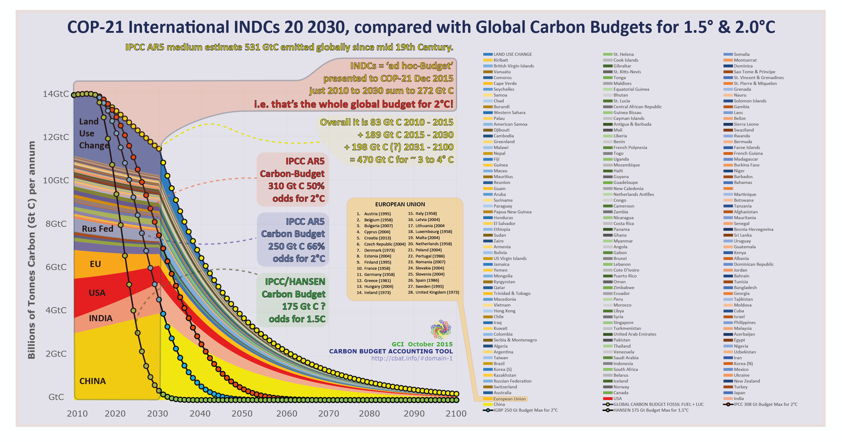
COP-21 said only 1.5°C to 2.0°C is policy relevant. The RCPs are 10% relevant at best, as they omit 1.5°C altogether and cover only 2.0°C to 10°C instead(!).
The RCPs formed the basis of the scientific guidance for Policy Makers in IPCC AR5. Carbon Budgets for 2.0°C are 437 Gt C and 4,500 Gt C for 10°C.
Aside from the 10% relevance above, the rest is misleading as both the assumptions and methodology behind the RCPs are wrong.
First it is not sensible to simply omit values for what you know you don't know. Second, including rates and ranges of impact that are unsurvivable is daft.
The 'RCP scenarios' are a classic expression of UKMO/IPCC under-estimating the extent and the risks of the climate change problem.
The INDCs to COP-21 are the mostly inadequate responses that reflect this, as they combine to doing much too little too late to avoid exceeding 2°C.
The 'Representative Concentration Pathways' [RCPs] are largely feedback-free having constructed and projected the unrealistic 100% 'sink-efficiency' by given dates.
They were executed on spreadsheets (not on expensive Super Crays) to give these results (see below).
They don't make physical sense as there is no understanding of real world 'feedback-process'.
Created by the UKMO and its colleagues elsewhere in IPCC, this methodology forms the basis of the 'policy guidance' given by IPCC in its '5th Assessment Report' (AR5) in November 2013.
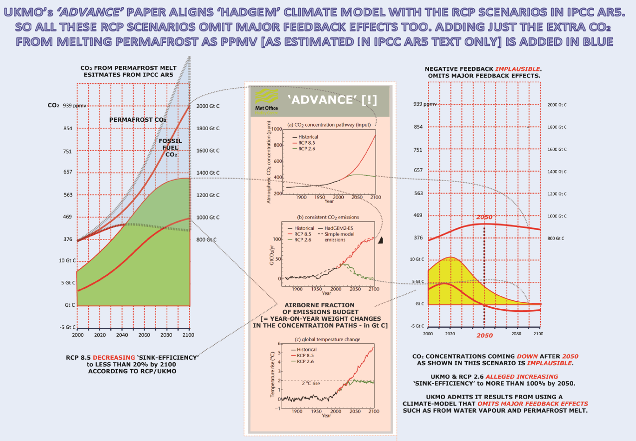
Bluntly, the RCPs omitted many significant feedback effects such as: -
- CO2 & CH4 emissions from permafrost melt,
- CO2 & CH4 emission consequent on albedo loss,
- water vapour, which can converted to 'CO2 equivalence'
- forest-burning (where land-sinks for CO2 convert to being sources)
- increased bacterial activity decomposing compounds contained in newly unfrozen soils and releasing CO2 & CH4,
- weakening of ocean sink due to increased acidification and temperature rise etc increasing atmospheric CO2 retention
- and the self-re-enforcing interactivity between effects such as these, contributing to the likely further acceleration of temperature rise & consequent rate of non-human CO2 release.
They were not candid about these omissions such as these in the RCP scenarios.
It is utterly inconceivable that PPMV C02 & W/m2 would or could go flat at the high-values/late-dates in RCPs shown here strongly but quite wrongly suggesting the achievement of 'equilibrium'.
At the very high levels 'modeled' they would continue to rise upwards due to the emssions and aggravated causation of the effects of the feedbacks.
'UKMO discreetly admitted' this in 2010, in a solitary unannounced (and recently changed - 2015) web-page (see pages 13 & 14) and here
In the climate change dynamics, amplifying feedbacks are like the black-holes of change, potentially drawing us over the climate-event-horizon.
Full set of RCP spreadsheets (2.5, 4.5, 6.0 & 8.5) were first distributed in May 2010
UKMO and colleagues elsewhere in IPCC collated and distributed this as follows: -
- RCP FINAL RELEASE, 26 Nov. 2009 (but see the spreadsheets themselves, as many date from earlier)
- RCP fait accompli from 2010 (UKMO)
- RCP fait accompli from 2010 (UKMO)
- 'Peer-Reviewed' acceptance only in August 2011
- Beginners Guide to RCPs in August 2013
- On June 12 2013 UKMO boasted to the EAC Enquiry in the House of Commons of, "providing more simulations to IPCC than any other group in the world"
Q61 EAC Carbon Budget and IPCC/UNFCC Enquiry Chaired by Joan Walley who asked UKMO: "How does that (scientific advice) relate to the IPCC?"
Professor Julia Slingo Director of the UKMO: "That process occurs every two years and of course we are a major player in the IPCC.
At the fifth assessment report we have a large number of contributing authors and we have probably contributed more model simulations than virtually any other group in the world,
so we take the IPCC process very seriously."
This UKMO RCP-methodology formed the basis of the 'policy guidance' given by IPCC in its '5th Assessment Report' in November 2013 to the UNFCCC.
An architect and independent voice from California, said this about the RCPs and the critique of its methodology, as analysed below: -
"I looked at the basis of their RCP scenarios and it is no wonder the UKMO can't model accurately or examine the 'big picture' feedbacks. There are four massive teams of folks each using different modeling programs with all kinds of data levels and physical measurement factors. The models each are too problem-centric to their own assumptions on all of this, plus they don't interact with each other (they can't).
And how do you correct the information in that much data? You can't.
The true test of this is that CBAT using the basic relational numbers from scientific data, has integrated the main climate drivers only, and is correctly estimating the actual ecosystems impacts that we've been seeing. It estimates these parameters very accurately, and is therefore a much better basis for global agreement structures.
The climate scientists are like the meteorologists trying to predict hurricane paths and strengths using about 20 different models and methods. Even those averages are frequently not accurate. As we've learned from the massive architecture and engineering platforms in microscopic detail, you can't really model reality, you can only come up with a real good guess. And that's where most of our client lawsuits come from now, the buildings don't perform as expected, too many systems and parts. It has to feed back from the owner's building systems engineer over a period of years and ADAPT THE MODEL TO FIT new detailed data. And that's just ONE building.
UKMO got off on the wrong foot by trying to minutely examine all physical factors in isolated models, a massive bureaucratic effort that will never "solve". Hence its serious inaccuracies over the last 20 years and is now completely missing the recently documented rapid warming generated by the feedback mechanisms (asymptotic, not linear). So they're clearly defending an inaccurate synthesis, as GCI points out
GCI's diagrams seem accurately to summarize this."What is clear is that while, "four quite separate and massive teams, each using different modeling programs with all kinds of data levels and physical measurement factors,"
the RCP scenarios all share the same calculating methodology shown below, so this obviously didn't happen by chance.
Probably around 2009 or even earlier, an agreement embedding a sequence of decisions, was made along these line: -
- DECISION ONE: scenarios each with the name of the W/m2 stabilisation level chosen. Hence RCP 2.5, 4.5, 6.0 & 8.5.
Then: -
- DECISION TWO: each team had instructions to proceed with: -
- DECISION THREE: ‘assert PPMV stability beyond date ‘x’’ in synch with the W/m2 stabilisation;
- DECISION FOUR: to compute carbon budget ‘y’ that gives; ‘z’, 100% sink-efficiency by date ‘x’
which is precisely what this analysis (with the weird carbon budget shapes in 4.5 and 6.0) reveals: - all have used the same calculation methodology.
Especially with all these different groups of people on the case, it is impossible for this - the same methodology across all four RCPs - to have occurred by accident.
Someone or some group agreed and then ensured that these instructions were followed.
There is a reasonable amount of evidence to support the the view that 'someone/group' was the UKMO or in the UKMO or linked to the UKMO.
However, UKMO ludicrously dispute all this and specifically all (what are their own) calculations below. So they have a problem.
As anyone who takes the trouble to look can see, these GCI calcuations faithfully and exactly reproduce the methdology and the data is in the spreadsheets they published in May 2010 that they now seek to refute.
Why would he or anyone do this? unless blinded by something undeclared, out of sight to all of us or something even worse and extremely foolish.
Representing UKMO, Richard Betts has persistently sought to deny the very existence of this methodology, effectively refuting the work of the UKMO or the group within/around it and in the IPCC.
It is part of their continuing attempt to conceal that the 'IPCC basis' of the policy guidance given UNFCCC was inadequate in that it was largely feedback-free. Why would he or anyone do this?After much resistance, and refusing point-blank to look at his own spreadsheets, he finally resorted to the defence of of this saying, 'what you say is there is there, but it is your perceptions of this which are wrong,' as though I was being asked to say whether his crown jewel was pretty or not.
Obvioulsy the frontier between climate science and climate policy is something of a serrated edge and if crossed by scientists, repositions them as policy actors.
The RCPs are policy and they became the basis of the policy-guidance in IPCC AR5, forming the backbone of the so-called 'Summaries for Policy Makers'.
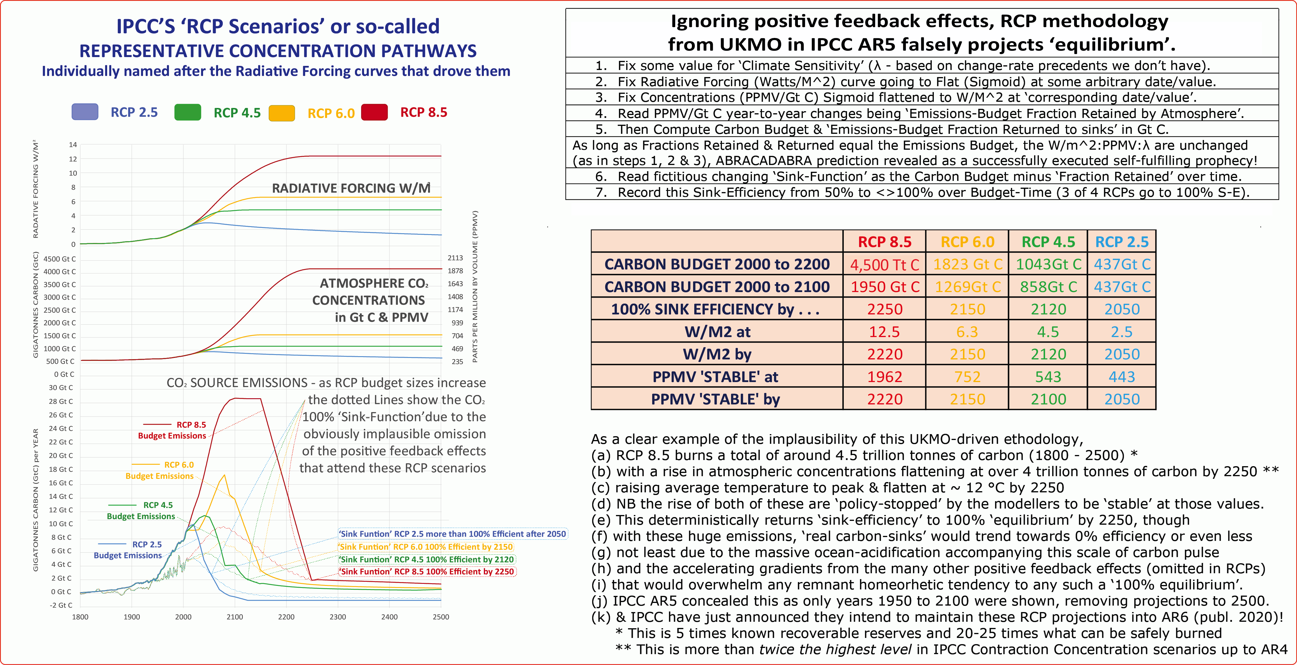
Chart One Top three RCPs clearly showing the modular calculations for the top: -[a] 3 CO2 concentration levels over time - the budget 'fraction-retained - to match the
[b] 3 watts/m2 levels for radiative forcing over time and
[c] 3 carbon budgets over time giving the
[d] 3 'sink-efficiency' levels - the budget 'fraction-returned, or budget minus fraction retained - where over time,
[e] annually the budget 'fraction-returned' equals the budget emissions themselves by a given date.
[f] & RCP 2.5 (the lowest) see chart 5 below.
Chart Two RCP 8.5 (Spreadsheets showing every detail of this is here)
[a] The CO2 concentration levels over time - the budget 'fraction-retained in the atmosphere - match
[b] The watts/m2 levels for radiative forcing over time and
[c] The carbon budget over time (here *over 5 times the known weight of recoverable fossil fuel reserves on the planet*) giving
[d] The 'sink-efficiency' levels - the budget 'fraction-returned (or budget minus fraction retained) - where over time,
[e] annually the budget 'fraction-returned' comes to equal the budget emissions themselves by and after a given date.
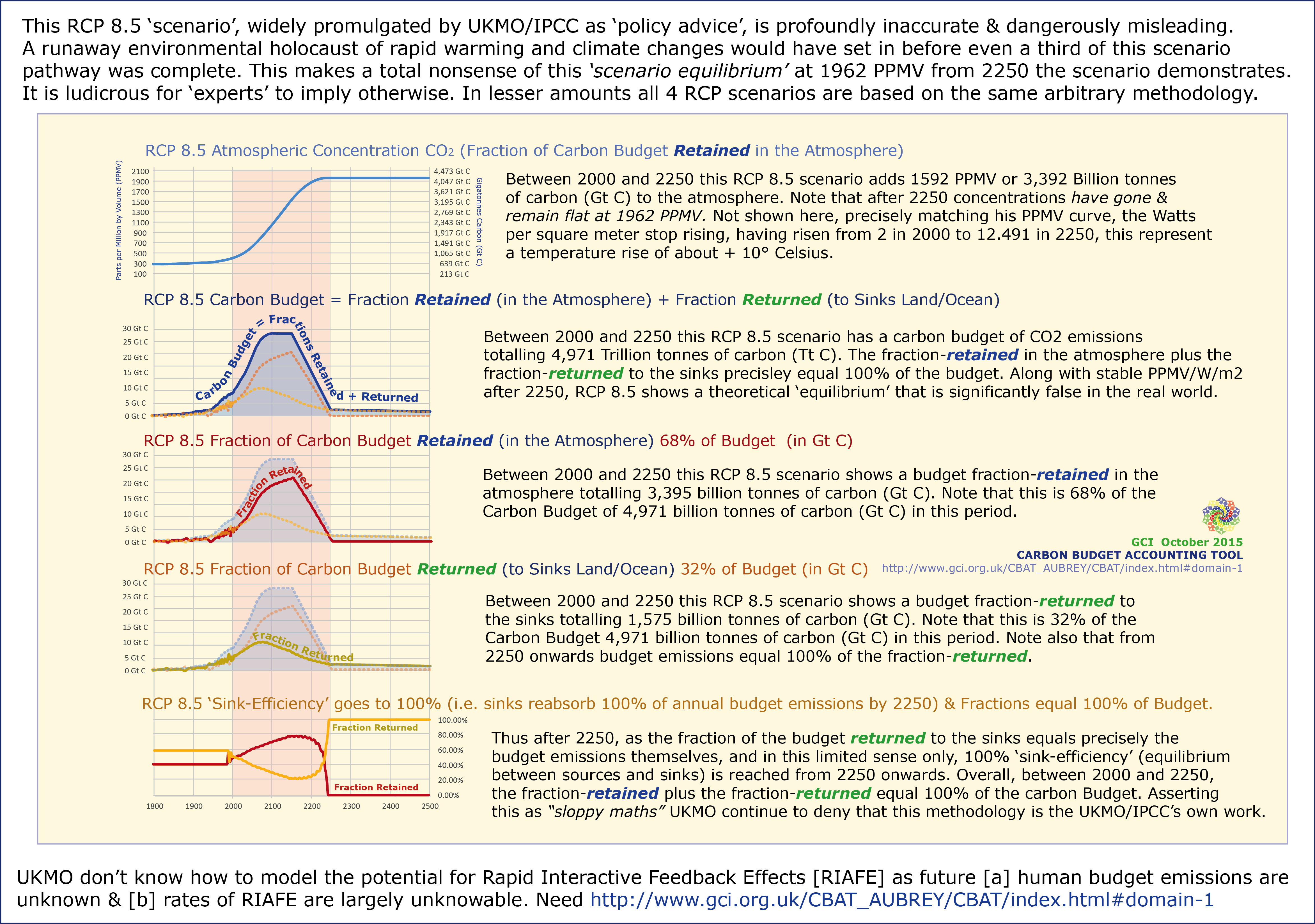
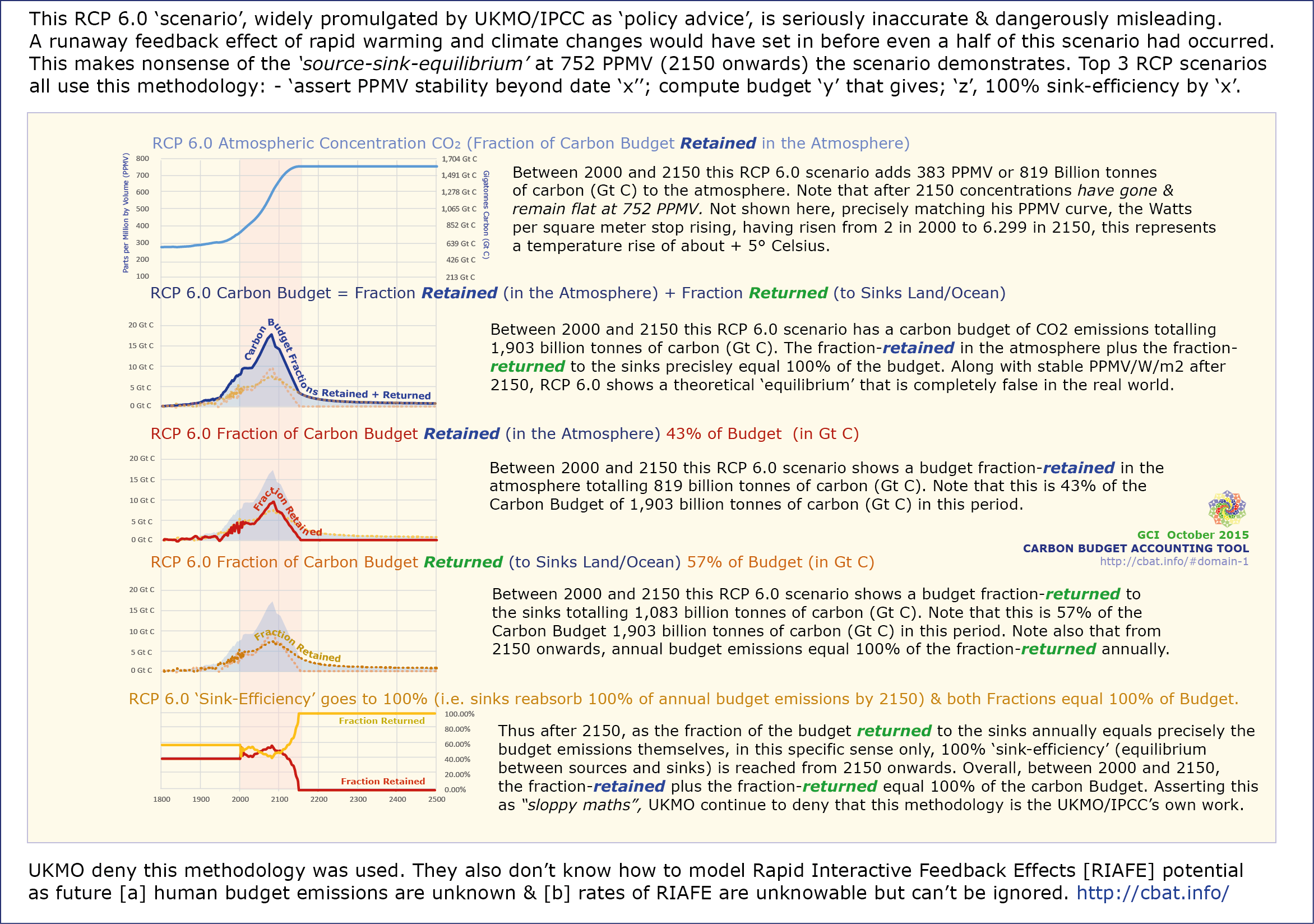
Chart Three RCP 6.0 (Spreadsheets showing every detail of this is here).
[a] The CO2 concentration levels over time - the budget 'fraction-retained in the atmosphere - match
[b] The watts/m2 levels for radiative forcing over time and
[c] The carbon budget over time giving
[d] The 'sink-efficiency' levels - the budget 'fraction-returned (or budget minus fraction retained) - where over time,
[e] annually the budget 'fraction-returned' equals the budget emissions themselves by a given date.
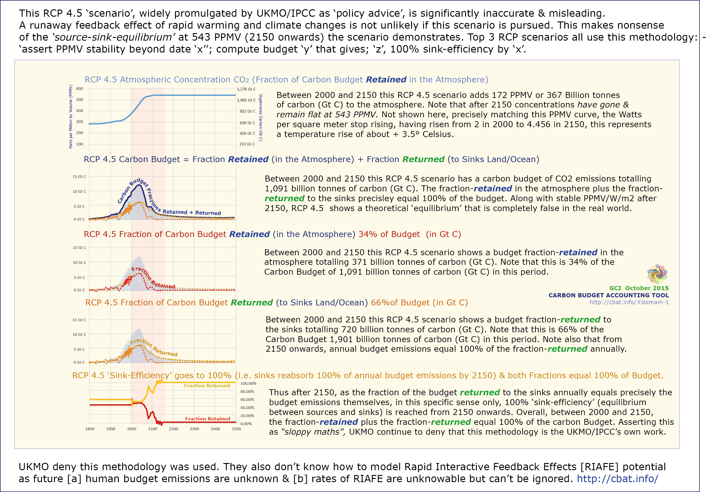
Chart Four RCP 4.5 - Spreadsheets showing every detail of this is here.
[a] The CO2 concentration levels over time - the budget 'fraction-retained in the atmosphere - match
[b] The watts/m2 levels for radiative forcing over time and
[c] The carbon budget over time giving
[d] The 'sink-efficiency' levels - the budget 'fraction-returned (or budget minus fraction retained) - where over time,
[e] annually the budget 'fraction-returned' equals the budget emissions themselves by a given date.
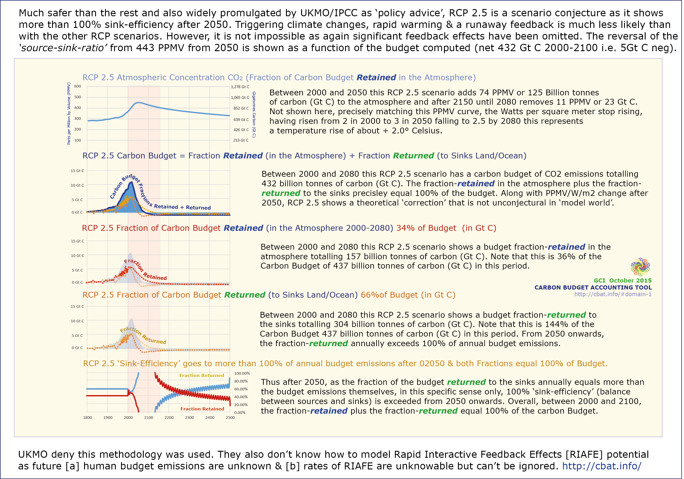
Chart Five RCP 2.5 - Spreadsheets showing every detail of this is here.
[a] The CO2 concentration levels over time - the budget 'fraction-retained in the atmosphere - match
[b] The watts/m2 levels for radiative forcing over time and
[c] The carbon budget over time giving
[d] The 'sink-efficiency' levels - the budget 'fraction-returned (or budget minus fraction retained) - where over time,
[e] annually the budget 'fraction-returned' exceeds the budget emissions themselves by a given date.
What this really means is that if the 'climate-modeling' fed into the IPCC by groups like UKMO over years past results in this sort of 'policy guidance', they now have a dwindling future as the policy-debate has begun and for UNFCCC-Compliance it is limited to IPCC for 2.0°C or Hansens' 1.5°C (confirmed at COP-21) & increasing anxiety over the issue of increasing feedback effects & the potential for runaway already at today's levels (2015).
As David King says here: -"DECC's GLOCAF is really an energy-policy model and I understand the need to include feedback-related emissions. It is important to deal with worst-case scenarios, and clearly this includes feed-back effects. At this point however, they are difficult to quantify or even estimate, however important. Converting this into impacts is what the ‘Carbon Budget Accounting Tool’ (CBAT) programme deals with and CBAT is obviously a great piece of work."
Especially in the light of the outcome at COP-21 (temperature between no more than 1.5° C-2.0° C)
What we need really need climate-science and modelling from RCP 2.5 downwards and not upwards (4.5 6.0 8.5) . . .
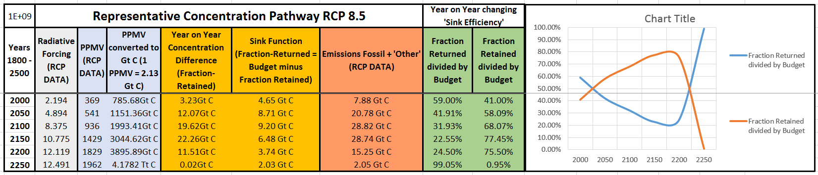
If a PPMV CO2 trajectory is projected into the future, then we can: -
- convert it to a weight Gt C
- measure year on year change in weight
- thus deriving (quantifying) the ‘sink function’ over that time period.
So: -
- when CO2 human-source-budget-emissions 'path-integrals' are projected into that future,
- we can measure the ‘sink-function’ (or efficiency’ of source:sink ratio) that has been assumed
- by comparing the two and quantifying these changes over time.
- As the RCP spreadsheet work above shows, doing this is very simple.
But: -
- in addition to that dynamic,
- arrays covering future potential feedback behaviours need to be included as well
- so CO2 non-human-source-emissions path-integrals are included and projected into that future,
- and we will need to adjust the reading of the sink-function to read for that extra contribution to the overall dynamic.
- This is less simple and the RCP spreadsheet work above effectively omits all of this.
Essentially, for this what we need to know is what: -
- arrays future human-source contraction-budget-emissions will be (NB these are more policy-relevant estimates)
- future non-human source CO2 equivalent feedback-emission (non-budget emissions)
- and knowing these will be at best just a bunch of best-guesses and thus
- what the future strength of the sink function might be in the face of that and
- how this may vary (accelerate/decelerate) over time in measurement arrays estimates.
For policy/strategy reasons 'rational-arrays' covering the potential for this are necessary and have been done.
In principle, to do this, all that is needed is: -.
Some basic data regarding: -At this stage what we don’t need is some Quaker Guns (deception) involving: -
- existing patterns of fossil fuel use and the airborne-fraction of this
- quantified emissions-scenarios or carbon-budget-projections (contraction-budget-emissions)
- some best guesses with 'trend-measurement' and some candour about
- feedback-knowns and unknowns
- while also allowing for unknown-unknowns . . . . . . . .
- and some arrays of trend-mesarement on spread-sheets (animated here)
- swarms of £100 million super Cray computers (UKMO) with huge fiscal overheads
- for bunches of cash-hungry guys posing as ‘experts’ to give us
- endless 100 year weather forecasts to discover 'the emergent properties of the models'
- to help disguise the core simplicity of the basic assumptions and trend-guesses
- while this same bunch of guys posing as experts and spending money hand over fist
- have actually made such assumptions/guesses using simple spreadsheets (not opaque and exorbitant GCMs)
- while pretending (ludicrously) that the 'sink-function' and 'climate sensitivity' are 'emergent properties of the GCMs' (sic)
- on the basis of omitted feedback emissions/effects and their inter-activity
- to actually get the completely deterministic & feedback-sparse RCPs that dominated the ‘policy guidance to the world from IPCC AR5
- which they then try and deny.
Whatever emerges, the message is the same,
- if we want to avoid dangerous rates of climate change,
- we must stop burning fossil fuel and putting more CO2 in the atmosphere as soon as is humanly possible.
- The danger or doing too little too late is a real pervasive and growing danger.
**********************************************************************************
What serious-minded people have said about climate models and feedback omissions . . .
David King - Former Chief Scientists & now Leading Government Climate Risk Programme at FCO
- Of course I understand the need to include feedback-related emissions.
- It is important to deal with worst-case scenarios, and clearly this includes feed-back effects.
- At this point they are however difficult to quantify or even estimate, however important.
- Converting this into impacts is what I assume the Carbon Budget Accounting Tool (CBAT) programme deals with.
- "It is obviously a beautiful piece of work."
Erica Thompson – GLOCAF team at Department of Energy & Climate Change
- Feedbacks likely unquantifiable until well after they are in full swing,
- at which point it is not a whole lot of use to quantify them.
- to such existential risks detailed future projections are largely impossible & potentially misleading because we are going so far out of sample,
- making it difficult to envisage any meaningful model calibration procedure.
- A qualitative exploration of the possible effects of different plausible feedbacks is perfectly sensible,
- Reliable quantitative projections seem to be unachievable.
- We don’t need reliable quantitative future projections to make sensible climate policy.
- Personally, I would advocate a precautionary approach
Dimitri Zenghelis, Alina Averchenkova & Nicholas Stern From LSE Grantham Centre on Climate Change
- The scientific models mostly leave out dangerous feedbacks/tipping points.
- At 6°, 5°, 4° C or below, the probability of passing some tipping points, such as melting of permafrost, may be high.
- If modellers cannot capture or model effects ‘sufficiently clearly’ they are omitted. Best guess surely not zero.
- We did run various scenarios which supported the broad conclusions of the paper
- One was precisely that the urgency of emissions reductions subject to growth & population projections swamps the distribution of ethical drivers
- It is important that we have the cited C&C numbers right.
- I have informed colleagues, including those at DECC, for whom your comments might help inform future runs of the GLOCAF model.
**********************************************************************************
